Introduction

Data is helpful for monitoring performance or changes on the dairy farm. One of the most common ways people analyze data is by calculating averages. Averages provide us with a quick, easy, and helpful snapshot of the data, but they aren’t perfect. Particularly, they don’t always reflect variation in data well. This gap can hide inconsistent or variable performance. To get a clearer picture of variability and performance on your farm, it is time to look beyond the average. 

This article explains when variability matters, how averages can fall short, how additional measures can improve data interpretation, and illustrates these concepts with examples using farm data.

Is Variability in My Farm’s Data Bad?

Variation is a normal part of any dataset. There is always some level of uncertainty or natural fluctuations that we cannot control. How much variability is considered “normal” depends heavily on the situation. For example, a tightly controlled laboratory experiment should have far less variation than observational data collected in a real-world setting like daily milk yields on a dairy farm. 

While farms can manage certain factors influencing animal performance, not all sources of variation can be controlled. Environmental conditions, animal behavior, health events, and genetics all contribute to natural variability. But reducing unnecessary variation can improve productivity, consistency, and economic outcomes. 

So, when does variation become a concern on a farm? There is rarely a black and white, universal cut-off. Instead, each farm should recognize its normal range of variation and identify when data begins to fall outside that expected range, whether due to controllable or uncontrollable factors. The following sections outline measures farms can use to evaluate and track consistency with their data. 

When The Average Falls Short

Averages are a powerful tool for summarizing data and are a cornerstone of most data analysis. However, averages don’t always tell us the whole story when discussing variability. 

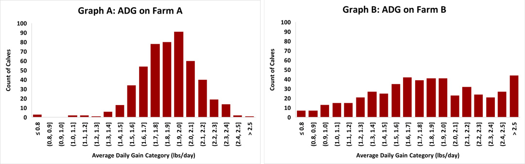
Averages can mask inconsistency in datasets [1]. For example, consider two farms tracking average daily gain (ADG) of calves from birth to weaning. Both report an average ADG of 1.85 lbs/day, suggesting similar performance. Curious if extreme outliers might be skewing the average, both farms also look at the median (the middle value of the dataset). Medians can provide a clearer picture when outliers influence averages. In this case, the medians are similar, 1.8 lbs/day for Farm A and 1.9 lbs/day for Farm B. 

But when we look at the distribution of the data (Graphs A and B), a different story emerges. On Farm A, the ADG values are closely grouped together, indicating less variation in calf growth. On Farm B the values are more spread out and not distributed evenly with some calves growing much faster and others much slower. This wider spread suggests less consistent growth on Farm B, even though their average ADG is the same as Farm A’s. 

Without examining the distribution of the data, Farm B may overlook the opportunity to improve calf growth consistency. For this reason, the average alone is not a perfect measure for tracking performance on dairies. 

Tools to Examine Variability

Understanding variability helps identify bottlenecks, inconsistent performance, or areas for improvement. While some variation is always expected and unavoidable, reducing unnecessary variation can be beneficial. There are three methods that when used together can elevate your data evaluations: 

1. Visualization
2. Standard deviation (SD)
3. Coefficient of variance (CV)

Note: While discussing these methods, it is important to remember that the amount of data affects how much variability may be observed. Smaller datasets tend to show more variability simple due to having fewer data points.

Visualization

Graphing data is a quick and simple way to assess how spread-out data is and to spot consistency patterns. The human brain can process visual information faster and more easily than statistical numbers, making graphs useful for understanding overall patterns in data [2]. They can also show trends or outliers that might not be clear from just looking at data, as mentioned in the previous section. 

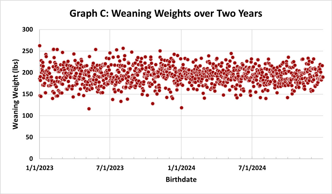
Scatter plots, bar charts, and other types of graphs can help visually highlight variation. However, differences in variability can sometimes be subtle. For example, when looking at a graph of weaning weights from the last two years for a farm (Graph C), there is a decrease in variability from Year 1 to Year 2. Although you may notice the subtle change visually, it’s hard to know how much it improved. That’s where it becomes helpful to pair data visuals with statistical measures that can provide clear, numerical measures of data variability. 

Standard Deviation (SD)

Standard deviation measures how far away data points typically are from the average [3].  

• Low SD = Data points are clustered closer to the average, implying less variability and more consistency. 
• High SD = Data points are spread out over a wider range, implying more variability and less consistency. 

For example, let’s revisit the earlier ADG comparison of Farm A and Farm B (Graphs A and B above). Farm A has a standard deviation of 0.2 lbs/day while Farm B has a standard deviation of 0.5 lbs/day. This confirms that Farm B’s growth rates are more widespread than Farm A’s, despite having the same average. 

Because SD is reported in the same units as the original data (i.e. pounds, dollars, inches), it is easy to interpret within a single dataset. However, because SD reflects the magnitude of the data, comparing across different data types can be difficult. For example, compare these two datasets: 

• Set A, Breeding Heifer Weights: Average = 800 lbs, Range = 700 to 900 lbs, SD = 40 lbs. 
• Set B, Calf Weaning Weights: Average = 200, Range = 150 to 250 lbs, SD = 20 lbs.  

Which of these datasets is more variable? Would you be surprised that it is Set B? Using a different measure, the coefficient of variation, is a helpful fit for answering questions like this. 

Coefficient of Variance (CV)

The coefficient of variance, usually reported as a percentage, measures the variability of data relative to the average.  Similar to standard deviation,  

• Low CV indicates less variation. 

• High CV indicates more variation. 

Because CV is a percentage value, it allows for easier comparison across different types of data (3). For example, let’s revisit the two datasets mentioned in the previous section:  

• Set A, Breeding Heifer Weights: Average = 800 lbs, Range = 700 to 900 lbs, SD = 40 lbs, CV = 5%. 

• Set B, Calf Weaning Weights: Average = 200, Range = 150 to 250 lbs, SD = 20 lbs, CV = 10%. 

The lower CV for the breeding heifer weights (5%) suggests that they are less variable than the calf weaning weights (10%). 

A challenge with CV is determining what level of variation is acceptable.  Acceptable thresholds depend on context and expectations. For example, a lower CV may be expected for a situation requiring precise measurements such as chemical concentrations used for cleaning protocols. Whereas a higher CV could be expected for measurements like calf birth weights.  

Because of this, CV is often most useful for benchmarking against yourself. This can help you monitor changes in variability, set expectations, and compare performance across years, seasons, or management changes. For example, if your typical CV for heifer weights returning from your custom grower is 15-25% and suddenly it increases 35% for several months, you can recognize that an issue may be occurring somewhere. Even if you already observed a management or consistency issue, CV can help quantify its impact. 

Bringing It All Together with a Real Farm Example

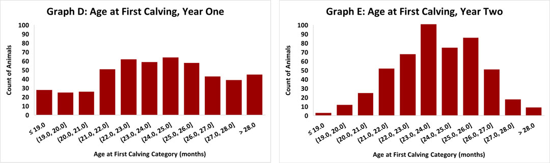
Age at first calving is a common metric for farms monitoring heifer reproductive programs. On E.X. Farms, the goal is for heifers to calve for the first time at 24 months of age. Let’s evaluate two years of data.

Year 1

The average age at first calving was exactly 24 months. Although this suggests they are achieving their goal, they chose to dig deeper. Graphing the data (Graph D) revealed a wide range of calving ages from under 19 months to over 28 months. The standard deviation was 3 months, and the coefficient of variance was 12.7%. In response, the farm focused on tightening their heifer reproduction protocols to reduce variability for year 2. 

Year 2

After Year 2, the average age at first calving was still 24 months. However, graphing the data (Graph E) showed calving ages more tightly clustered around the target. To quantify this improvement, they recalculated the standard deviation and coefficient of variance. The standard deviation had decreased to 2 months and the CV to 8.5%, confirming that they had decreased the variability of their herd’s age at first calving. 

Author

References

- Kotronoulas, G., Miguel, S., Dowling, M., Fernandez-Ortega, P., Colomer-Lahiguera, S., Bagcivan, G., Pape, E., Drury, A., Semple, C., Dieperink, K., & Papadopoulou, C. (2023). An overview of the fundamentals of data management, analysis, and interpretation in quantitative research. Seminars in Oncology Nursing, 39(2). https://doi.org/10.1016/j.soncn.2023.151398
- Franconeri, S.L., Padilla, L.M., Shah, P., Zacks, J.M., & Hullman, J. (2021). The science of visual data communication: What works. Psychological Science in the Public Interest, 22(3), 101-161. https://doi.org/10.1177/15291006211051956
- Siegel, A.F. (2016). Variability: Dealing with diversity. In Practical business statistics (7th ed.) (pp.101-128). Elsevier Inc. https://doi.org/10.1016/B978-0-12-804250-2.00005-5