Most dairy farms today collect data by which they attempt to make informed decisions about how to manage their herds. There is an adage:
If you can’t measure something, you can’t monitor it. And if you can’t monitor it, you can’t measure it.
The collection and interpretation of herd-level data is a positive trend throughout the dairy industry. The problem is there are many types of data, and a good manager must understand the nature and limitations of the types of data being monitored to make informed decisions.
Reproductive data is particularly difficult to measure which makes it a challenge to measure and monitor, even on large dairy farms. Measuring reproductive performance is about measuring probabilities—the likelihood an event will occur. Unfortunately, the human brain is not very good at comprehending probabilities. Further, the nature of reproductive data involves a frustrating factor called randomness; hence the title of this fact sheet: The Randomness of Reproduction. The following points need to be considered and understood so good managers do not fall into incorrect conclusions about the reproductive data they collect on their farm.
Understand the type of data being monitored
Data collected on dairy farms can generally be classified into two types: continuous variables versus categorical variables.
Continuous variables have an infinite number of possible values that fall between two extremes. Some examples of continuous variables measured on dairy farms are milk production, body weight, and feed intake. The critical point about continuous variables is measuring them requires a relatively small number of observations. Scientific experiments designed to detect the effect of feeding a certain diet on milk production can be conducted and validated on small numbers of cows. Further, these variables tend to fluctuate by small degrees.
Categorical variables differ in their nature from continuous variables. Most reproductive outcomes measured on dairy farms are a specialized subset of categorical variables called binomial variables. Binomial variables have only two possible outcomes. Most reproductive variables of interest on dairy farms are binomial in nature. Some examples of binomial reproductive outcomes include pregnancy outcomes (pregnant vs. open), pregnancy loss (yes vs. no), calf sex (heifer vs. bull), and twinning (singleton vs. twin). The challenge as we shall see with binomial variables is that, by their nature, they are susceptible to randomness.
The Law of Large Numbers
Jacob Bernoulli (1655–1705) was one of many prominent mathematicians in the Bernoulli family. His most important contribution was in the field of probability where he derived the first version of the Law of Large Numbers in his work Ars Conjectandi. As an illustration of the Law of Large Numbers, suppose 60% of the voters in Basel, Switzerland support the mayor. How many people must you poll for the chances to be 99.9% that you will find the mayor’s support to be between 58% and 62%? The answer that Bernoulli derived from his mathematics was 25,550 people—more than the entire population of Basel in Bernoulli’s day. Today, we can achieve a statistically significant result with an accuracy of +/– 5% by polling only 370 people. The problem is most dairy farmers succumb to the Law of Small Numbers, which is the misconception that a small sample accurately reflects underlying probabilities. It is a misguided attempt to apply the Law of Large Numbers when the numbers are not large.
Coin flipping
Think of a coin flip in which the two possible outcomes are either heads or tails. Most people know intuitively the chances of getting a head or a tail in a coin flip are 50:50. The mathematical problem, however, is to determine how many times I must flip a coin to prove that the odds of getting a head or a tail are 50:50.
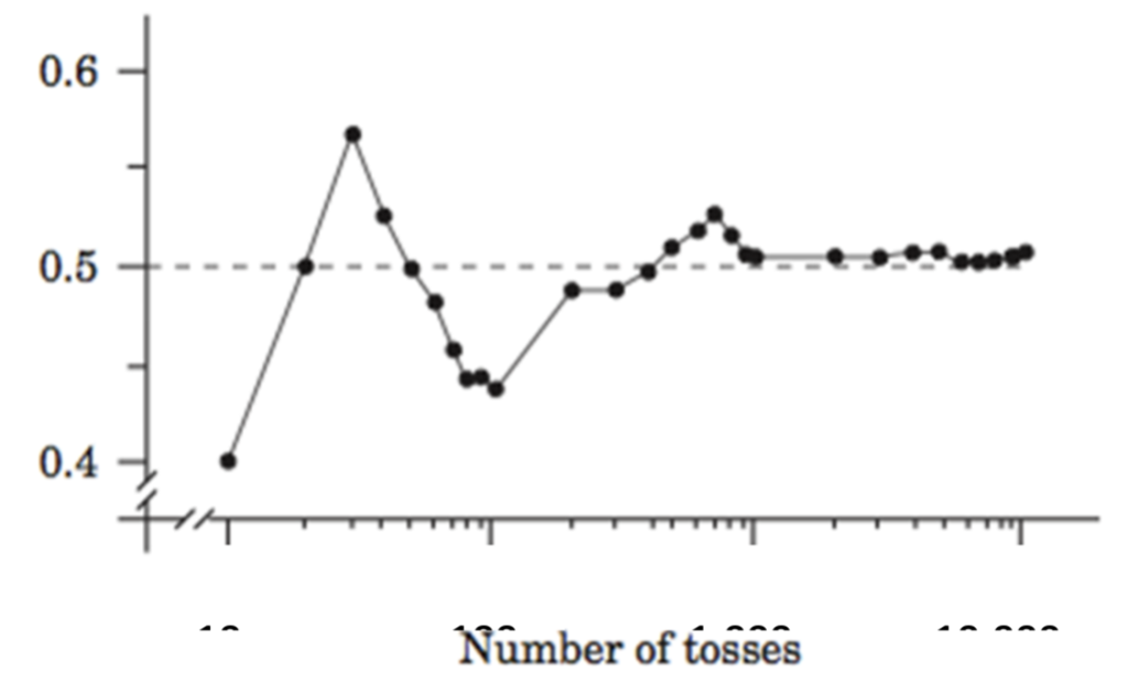
John Kerrich (1903–1985) was a mathematician who performed a famous coin-flipping trial illustrated in Graph 1.
A total of 10 or 100 flips did not approximate the expected outcome of 50% heads. It was not until he flipped his coin 1,000 times that the odds of getting a head approximated 50%.
Think of each individual cow at a herd check as the outcome of a coin flip. Most farms check far fewer than 1,000 cows at a given herd check. The problem with measuring a binomial outcome such as a pregnancy diagnosis is, by nature, you need a lot of observations to approximate the actual conception rate in a herd. Further, if you base conception rate on too few observations, you introduce a lot of random noise in the outcomes, which introduces variability that is difficult to distinguish from the actual value you are trying to measure.
The perils of “good” vs. “bad” herd checks
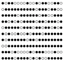
Consider Figure 1 which is a visual representation of the outcomes of 200 pregnancy diagnoses. White circles represent pregnant cows and black circles represent open cows.
In this example, the “true” conception rate for these 200 cows is 30% (60 pregnant out of 200 total). The problem is pregnancy outcomes are subject to the Law of Large Numbers, and most farms succumb to the Law of Small Numbers.
For example, a farm may have only 40 cows to check at a given herd check. If the subset of 40 cows checked are represented in the figure by lines 2 and 3, then the conception rate for that weekly herd check is only 9/40 or 23%. By contrast, if the subset of 40 cows checked are represented in the figure by the bottom two or top two lines, then the conception rate for that weekly herd check is 16/40 or 40%. If a herd only checks 20 cows weekly, then you can calculate the weekly conception rate for yourself. As you will see, the Law of Small Numbers introduces a lot of variability in the weekly herd check outcomes. In my experience, both veterinarians and farmers find this level of variation to be disconcerting to say the least.
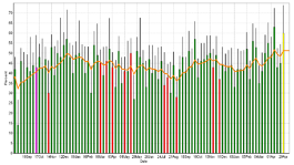
Graph 2 shows the weekly conception rate outcomes for a 3,000-cow dairy. You can see how the randomness of this binomial outcome affects the variability in herd checks from week to week. I was sent this graph from a farm who told me they were trying to deal with a high degree of weekly variation in pregnancy outcomes. They were frustrated by this apparent variability and wanted to know what was causing it. We now know this is the nature of measuring pregnancy outcomes which represent the variability typical for a binomial outcome. I can give many other examples of farms that have struggled with what they perceive to be more than the expected number of bull calves born in a given period of time or the sporadic nature of twin births. All these reproductive outcomes illustrate the Randomness of Reproduction that is inherent in measuring binomial outcomes.
What can we do?
The best we can do with reproductive data is to understand its limitations and how we interpret the outcomes. It is human nature to look for patterns and to assign them meaning when we believe we find them. In each case, the longer the sequence, or the more sequences you look at, the greater the probability that you’ll find every pattern imaginable— purely by chance.
I encourage dairies to collect reproductive data but to understand the difficulties in measuring reproductive outcomes. Understand that the outcome of weekly herd checks is going to be inherently variable. Do not panic if a weekly herd check is worse than expected. A better approach is to monitor changes across time.
Graph 2 includes a yellow line that is a mathematical average. This weighted average can be tracked over time to “smooth out” the weekly variation in pregnancy outcomes. Finally, larger dairy farms with more data have less weekly variability than small farms with fewer cows. While unfortunate, that is the nature of reproductive outcomes. Finally, even the largest farms will have some degree of variability in reproductive outcomes due to the Law of Large Numbers.
In the end, the Randomness of Reproduction is something that we all must learn to deal with and understand when interpreting reproductive data on dairy farms.
Developed by UW–Madison Department of Animal and Dairy Sciences Professor & Extension Dairy Reproductive Specialist Paul Fricke for the 2022 Badger Dairy Insight Webinar Series: The Randomness of Reproduction, March 29, 2022. Adaptation of this article printed in Hoard’s Dairyman, May 10, 2022.
The Drunkard’s Walk: How Randomness Rules Our Lives was the source for Figures 1 and 2 and the examples of Jacob Bernoulli and John Kerrich given in the May 2022 article, “The randomness of reproduction,” found on page 275. That book was published in May 2009 by Vintage Books, a Division of Random House Inc., New York, N.Y.


